Get Started with Scikit-Learn: A Machine Learning Guide

Scikit-learn, sometimes referred to as sklearn, is a Python machine learning framework that simplifies and speeds up the process of mining and analyzing data. It is extensively used in business and academics and has established itself as a potent, approachable machine learning tool. One of the most significant advantages of using sklearn is that it’s freely available for usage, modification, and distribution thanks to its permissive BSD license.

This getting started guide will discuss the basics of machine learning and how to implement it using sklearn. Since this is a beginner-friendly guide, it will be a bit long. So feel free to take your coffee breaks in between reading, or you can pause somewhere and come back later. That’s why it’s important to know how we’ve organized the article, and that’s what you’ll find in the next section (this can also be found briefly in the table of contents).

How you can get the best from this guide

This article is perfect for you if you are a beginner. However, even if you’re a pro, you can brush up on some of your concepts by reading. In addition, it will give you a good idea of using sklearn for machine learning problems. We’ve structured the article in the following way:

First, we introduce the concept of Machine Learning to you; specifically, we talk about the types of machine learning. In these sections, we also introduce you to the tasks you can perform with machine learning and the algorithms that help you accomplish them. If you know the basics of machine learning, feel free to skim through or skip it altogether.

After that, we talk about sklearn. In particular, we provide instructions for how you can install it as well as list the supported machine learning algorithms that you can use with sklearn.

Finally, we come to the third and most important part. In this part, we dive deep into how you can use sklearn to implement the machine learning concepts discussed in previous sections. We mainly focus on classification and regression problems using different algorithms and a beginner-friendly dataset (Iris dataset).

Now that you know this guide’s outline, we can start with the first part. Let’s talk about machine learning for a moment before moving on to how sklearn fits into the process of machine learning. Here, the concept of machine learning will be broken down for you, along with some popular examples.

What is Machine Learning or ML?

Machine learning, or ML for short, is a subfield of artificial intelligence concerned with creating algorithms and models that can learn from data and improve their predictions over time.

A dataset including both input data and labels is the general starting point for the machine learning process. The objective here is to build a model that, given the input data, can correctly predict the labels. For example, if a machine learning model were given a dataset of images labelled “cat” or “dog,” it could use this information (e.g., the shape of the ears, texture of the fur) to determine whether or not a new image fit into one of these categories. In order to train a machine learning model, we feed it input data and allow it to uncover relations that exist between the data and output labels. After the model has learned these correlations, we may use them to make predictions for new and unseen data.

Types of Machine Learning

Machine learning can be divided into two major groups: supervised learning and unsupervised learning. In supervised learning, the goal is to predict the labels of new examples. The supervised learning models are trained by utilizing examples that have already been labelled. In the previous section, the example of dog vs cat image classification would fall under supervised learning. When the model is given data without any labels, it is called unsupervised learning, and its purpose is to find patterns or structures in the data. There is also another popular form of machine learning called reinforcement learning. It is also commonly referred to as RL. An agent acquires knowledge through experience and the reinforcement (or lack thereof) it receives from its surroundings. In simpler terms, in RL, a system or model learns through feedback. For instance, if you give food to a dog only when it sits down, you are training it to sit whenever it wants food, thus positively reinforcing its behavior. This technique can also be used to learn complex behaviors in the context of games or simulations, as well as to solve control problems like the operation of a robot or autonomous vehicle.

Given that the sklearn package only supports supervised and unsupervised learning and does not have any implementations of reinforcement learning methods, we will concentrate on the former two. Let’s dig deeper into these two topics right now.

Supervised learning

As I told you earlier, the training data is labeled in supervised learning. This will become clearer with a real-life scenario where supervised learning is used.

Supervised learning: An example

Spam detection: An email service provider or application will often employ a supervised learning algorithm to analyze hundreds of emails’ metadata, such as the sender’s address, subject line, and body, and train itself so that it can determine if a new incoming message is spam. For this purpose, a model is trained using a dataset of previously labelled examples of emails which are divided into “spam” and “not spam” classes.

Supervised learning: Tasks

Now that you know what supervised learning is, it’s time to discuss some of the jobs it is used for.

• Classification: The term “classification” refers to the procedure by which it is decided whether or not a newly collected sample should be categorized as, for example, “cat” or “dog” based on physical features such its color, size, and shape. This has applications in areas like spam detection (as discussed earlier) and credit fraud analysis (predicting whether a transaction is fraudulent or not).
• Regression: It is the method of forecasting a variable (such as price or temperature) for a new example based on previous examples’ characteristics like size, location, and age. One application of regression is to estimate a home’s value in relation to its area (in square ft.), neighborhood, and other characteristics. A second illustration would be using regression to assess the fuel economy of a vehicle on the basis of its specifications.
• Time series forecasting: The term “time series forecasting” is used to describe the procedure of making predictions about the value of a target variable at a later time using data from the past. This can be put to a number of different uses, such as predicting future stock prices for a company or estimating future product demand from existing data.

Supervised learning: Algorithms

What are some of the supervised learning algorithms for accomplishing those tasks? Let’s take a look: (Don’t worry if you don’t understand everything you read here. It can be a bit overwhelming if you’re just starting; however, you’ll soon get a hold of these concepts once you are more familiar with them.)

• Linear regression: A straightforward and common approach to the problem of regression, linear regression is based on the assumption that the connection between the data to be analyzed and the desired outcome is a straight line.
• Logistic regression: The term “logistic regression” refers to a model for classification problems, which is both straightforward and quite popular. This model makes use of a logistic function to estimate the chance that a new example belongs to a particular class. After that, it places the example in the category that has the greatest probability.
• Support vector machines (SVMs): They are a powerful and versatile model that can be used for classification and regression tasks. This model searches for the hyperplane in the feature space that either separates the classes as much as possible (for classification) or minimizes the error (for regression).
• Decision trees: They are a type of tree-based model that can be used for classification and regression tasks. This model recursively partitions the data into subsets depending on a feature value test. The values of the tree’s leaves are used as predictions.
• K-nearest neighbors (KNN): It is an easy-to-use and effective model for classification and regression problems. It makes predictions based on the labels of the nearest neighbors in the training set. The user decides the number of neighbors – a hyperparameter for this model.

Unsupervised learning

As the name suggests, the training data has no labels in unsupervised learning. Let’s look at a real-life usage scenario for this type of machine learning.

Unsupervised learning: An example

Customer segmentation or market segmentation is the process by which a company splits its customers into distinct categories to classify customers based on their buying habits or many other similar parameters. This is a scenario where unsupervised learning algorithms can be used. The algorithm is not given any labels; instead, it searches for patterns in the data to identify clients with similar tastes. An example of this would be e-commerce sites. These sites use your previous browsing and buying records to suggest products that match your interest, which greatly improves the odds of you making a purchase.

Unsupervised learning: Tasks

The goal of unsupervised learning is not to make predictions about the labels of new examples but rather to find relationships or structures in the data. Some examples of unsupervised learning tasks include:

• Clustering: It is a type of unsupervised learning task that necessitates partitioning the data into groups (sometimes called clusters) based on similarity.  The process of clustering can be utilized to uncover natural groupings within the data and has applications in areas such as consumer segmentation and the detection of anomalies.
• Dimensionality reduction: This is an unsupervised learning process that entails lowering the number of features in the data while keeping as much information as is possible. It is possible to discover essential features and compress data for storage or transmission using this technique.
• Anomaly detection: Detecting anomalies is an unsupervised learning task that requires finding samples within the data that do not conform to the expected pattern or behavior. An anomaly is defined as something that deviates from the norm. For example, an uncommon occurrence, fraudulent activity, or data inaccuracy could all be uncovered with the use of anomaly detection.

These are just a few examples of unsupervised learning tasks. There are many other types of tasks that can be addressed using unsupervised learning.

Unsupervised learning: Algorithms

The following are some examples of algorithms that are used in unsupervised learning:

• K-means clustering: This is a technique that splits the data into a predefined number of clusters based on how similar the cluster members are. It does this by iteratively assigning each example to the cluster with the nearest mean and then updating the means to the centroid of the new clusters.
• Hierarchical clustering: It is a type of clustering algorithm that generates a hierarchy of clusters by iteratively merging clusters that are the most similar to one another. Hierarchical clustering can be broken down into two primary categories: agglomerative and divisive. Agglomerative hierarchical clustering begins with individual examples and then combines them into clusters; divisive hierarchical clustering begins with the entire dataset and then divides it up into smaller clusters.
• PCA: Principal component analysis, also known as PCA, is a type of dimensionality reduction method that projects the data onto a space with fewer dimensions. This is accomplished by determining the directions in which the data exhibit the greatest amount of variance.
• Autoencoders: They are a type of neural network architecture that consists of both an encoder and a decoder.   The encoder maps the input data to a lower-dimensional representation, which is used by the decoder to reconstruct the original data. Dimensionality reduction and feature learning are two applications that are possible uses for autoencoders.

Sklearn

If you have been reading attentively, you have a general idea about Machine Learning. Now let’s get back to our main focus – sklearn. First, I will tell you how to install sklearn.

Sklearn: Installation

To get scikit-learn up and running, you’ll need to install Python and the Python package management, accessed by the pip command. You can install scikit-learn by typing the following command into the terminal:

pip install scikit-learn

Doing so will get you the most recent version of scikit-learn and any other required libraries onto your machine. Alternatively, the conda package manager included in the Anaconda distribution can be used to install scikit-learn. Use the following command to install scikit-learn with conda:

conda install -c anaconda scikit-learn

By running the previous command, you can have scikit-learn and all of its prerequisites added to your conda installation. After installing scikit-learn, you can verify whether it was installed successfully by importing it in your Python code with the “import” keyword. The import statement you should use is the following:

import sklearn

Scikit-learn provides a set of tools for creating and analyzing machine learning models. Installing sklearn may have failed if you receive either “ImportError” or “ModuleNotFoundError: no module named “sklearn”” message.

Sklearn: Supported algorithms

Let’s take a look at some of the algorithms that are supported by sklearn (I will not list any algorithms that have not been discussed in this article):

• Classification algorithms:
  • Logistic regression
  • Support vector machines (SVMs)
  • K-nearest neighbors (KNN)
  • Decision trees

• Regression algorithms:
  • Linear regression
  • Support vector machines (SVMs)
  • K-nearest neighbors (KNN)
  • Decision trees

• Clustering algorithms:
  • K-means
  • Agglomerative clustering

• Dimensionality reduction algorithms:
  • Principal component analysis (PCA)

Sklearn is compatible with the aforementioned set of algorithms for different tasks. I have only touched on a few of the more well-known varieties in the above list. Sklearn also has a wide variety of utility functions and algorithms that can be used in various phases of machine learning implementations and processes.

Machine Learning with Sklearn

Now that you have a basic understanding of Machine Learning and Sklearn, let’s move on to the main part of the article – machine learning with sklearn. We’re going to cover 3 tasks with sklearn: 1) Classification, 2) Regression, and 3) Clustering. You already have a basic idea of what they are. So let’s begin to dive deep.

Classification

Classification is a supervised learning task that involves predicting a class label for a brand-new example based on the class labels of a training set. The goal of classification is to establish a link or a relation between the input data and the labels produced.

Think about a set of customer data that includes specifics about each client’s age, income, and location. A classification model may be able to predict if a new consumer would buy a product in the future if their age, income, and location are known. In this case, the class labels would be “buy” and “not buy,” and the input data would be the customer’s age, income, and location.

Other classification jobs include detecting spam, looking for credit fraud, classifying images, etc. As you’ve already seen, various methods can be used for classification, including support vector machines, decision trees, logistic regression, and k-nearest neighbors. The nature of the data and the job’s requirements determine which algorithm is used.

Classification dataset: Iris dataset

You’ve probably understood so far that we need a labeled dataset to try the problem of classification. We’ll use the Iris dataset for this purpose.

The Iris dataset is a famous dataset in machine learning and is frequently used as an example in machine learning lessons for beginners. It comprises 150 observations of iris flowers, with four characteristics for each flower recorded in centimeters: sepal length, sepal width, petal length, and petal width. Each observation is labeled with the species of iris flower to which it corresponds: Iris setosa, Iris versicolor, or Iris virginica.

We’ll show you what this dataset looks like as we dive into the programming bit in the next section.

Classification with sklearn

We’ll start coding from here. As you already know, we have a multitude of algorithms to choose from for classification. Let’s start with the logistic regression.

Logistic regression

First, we need to import the necessary modules and load the Iris dataset (If you don’t have any of the modules listed here, you can easily install them using pip):

Note: If you have Jupyter notebook installed, it would be easier for you to follow along since it lets you run code in sections.

import numpy as np
import pandas as pd
from sklearn import datasets
from sklearn.model_selection import train_test_split
from sklearn.metrics import accuracy_score
from matplotlib import pyplot as plt
%matplotlib inline

# Load the Iris dataset
iris = datasets.load_iris()
X = iris["data"]  # input features
y = iris["target"]  # labels

# Copy the dataset to a pandas DataFrame
df_iris = pd.DataFrame(X, columns = ['Sepal_length','Sepal_width','Petal_length','Petal_width'])
df_iris['labels'] = y.tolist()

I’ve imported specific models from the sklearn package because we only need specific items. Then I loaded the Iris dataset that is included in the sklearn package. I assigned the “X” variable for the input features of the dataset and “y” for the labels. I’ve also copied the dataset to a data frame, as you can see. Run the code. Now let’s take a look at how the Iris dataset looks like using the following piece of code:

df_iris.head()

After running it, you will be able to see the first 5 examples of the dataset:

	Sepal_length	Sepal_width	Petal_length	Petal_width	labels
0	5.1	3.5	1.4	0.2	0
1	4.9	3.0	1.4	0.2	0
2	4.7	3.2	1.3	0.2	0
3	4.6	3.1	1.5	0.2	0
4	5.0	3.6	1.4	0.2	0

In the first 4 columns, you can see the values of “X” or the input features. In the labels column (“y”), you can see all are 0, which is the number set for Iris setosa. If you look at the tail end of the dataframe, you will see all labels are 2, indicating Iris virginica. Label 1 is set for the Iris versicolor.

Now there are 150 examples in this dataset. We could use all of these examples to train a machine learning model that will find the connections between the input features (4 features: Sepal_length, Sepal_width, Petal_length, Petal_width) and the labels or the species of Iris. However, we must not use all 150 examples for training purposes. Why? Because we also want to test whether our model accurately predicts when it is fed with some new data. That is why we will split the dataset into two sets for training and testing purposes using the Sklearn train_test_split() method:

# Split the dataset into a training set and a test set
X_train, X_test, y_train, y_test = train_test_split(X, y, test_size=0.5, random_state=22)

Here, the “test_size” parameter is used for determining the size of the test dataset. As it is set to 0.5, it will store half of the dataset or 150/2 = 75 examples in the test dataset (X_test, y_test). The other 75 examples will be in the training set (X_train, y_train). Now, there is another parameter that you might have noticed. It is the “random_state” parameter. Why do we use this? We need to randomize the dataset and then split it into training and testing dataset. This is because if only the first half of the dataset is stored in the testing dataset, then we will not get any examples with label “3”. When the random_state parameter has a certain integer value assigned to it, the random shuffling will always result in the same pattern. If the random_state is not set, then each time the code is run, it will generate different random datasets each time.

Now, we will use the “LogisticRegression” model from sklearn to train our classifier:

from sklearn.linear_model import LogisticRegression

# Train a logistic regression classifier
clf = LogisticRegression(max_iter = 300)
clf.fit(X_train, y_train)

LogisticRegression
LogisticRegression(max_iter=300)

We’ve set the maximum iterations for the regression to be 300. If you encounter an error saying “STOP: TOTAL NO. of ITERATIONS REACHED LIMIT,” increase this value to increase the maximum number of iterations. Running the previous snippet of code will train our classifier model. Now it’s time to test how well the trained model performs.

# Make predictions on the test set
y_pred = clf.predict(X_test)

# Compute the accuracy score
accuracy = accuracy_score(y_test, y_pred)
print("Accuracy:", accuracy)

Running this bit of code will use our trained model to make predictions (y_pred) on the new examples or the testing dataset (X_test). It will also calculate the accuracy of the model using the actual labels (y_test) and the predicted ones (y_pred).

Accuracy: 0.96

Let’s understand what this means in more detail. Write the two lines of code below and run it:

print("Actual labels:", y_test)
print("------------------")
print("Predictions:", y_pred)

Actual labels: [0 2 1 2 1 1 1 2 1 0 2 1 2 2 0 2 1 1 2 1 0 2 0 1 2 0 2 2 2 2 0 0 1 1 1 0 0
 0 2 2 1 1 0 0 1 1 2 2 0 1 1 2 0 0 0 0 0 0 2 1 1 2 0 0 0 0 1 0 1 1 1 1 1 0
 1]
------------------
Predictions: [0 2 1 2 1 1 1 2 1 0 2 1 2 2 0 2 1 1 1 1 0 2 0 1 2 0 2 2 2 2 0 0 1 1 1 0 0
 0 2 2 1 1 0 0 2 1 2 2 0 1 1 2 0 0 0 0 0 0 2 1 1 2 0 0 0 0 1 0 1 1 1 1 2 0
 1]

As you can see, we have printed “Actual labels” and “Predictions,” and the predictions are mostly accurate.

How it works:

To understand how the logistic regression classifies between 3 categories of Iris flower species, you can look at this here: https://scikit-learn.org/stable/auto_examples/linear_model/plot_iris_logistic.html

I will copy the figure from the webpage here and explain how the logistic regression 3-class (for 3 class of flowers or labels) classifier works:

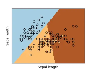
Here, only 2 input features were used to train and test the model: Sepal width and Sepal length.

Generally, logistic regression works on binary classification problems (problems that only have 2 classes or 2 types of labels). However, it can be used for multiclass classification (the Iris dataset has 3 classes, making it a multiclass problem), which is accomplished by training multiple binary classifiers, one for each category. In sklearn, you don’t have to specify anything for multiclass problems. It will automatically detect the number of classes and apply logistic regression. There is a parameter for modifying the multiclass logistic regression named “multiclass.” It has a default value set to “auto”, which allows it to use multiclass approach when necessary. In brief, it’s a linear model, and as you can clearly see from the figure, the model, in essence, figures out the straight lines that separate the three categories of flowers.

Now that you’ve learned how to apply logistic regression with sklearn, let’s see some other algorithms that you can use. If you’ve understood how we applied logistic regression to our dataset, then you can apply the other algorithms easily. Let’s go over them very briefly so you can figure out the rest and try them on your own.

K-nearest neighbors (KNN)

K-Nearest Neighbor (KNN) is a straightforward approach to classification. Labels are used to categorize training data into separate groups. After being trained, a KNN model may take an unseen sample and assign it to the cluster that contains the most similar data. Rather than actively developing a model, this algorithm just saves the training data and uses the similarities between a new sample and the stored data to predict the label of the new sample. This enables it to provide reliable predictions in situations when there is a lot of data.

Let’s use the same Iris dataset to classify the 3 flower species, this time using KNN. You don’t need to modify much of the previous code that we used for logistic regression. You only have to import the KNN model and apply it instead of applying logistic regression.

Now, replace the previous code section “# Train a logistic regression classifier” with the following code, which will import the KNN model and fit it to our dataset:

from sklearn.neighbors import KNeighborsClassifier

# Train a KNN classifier
knn = KNeighborsClassifier(n_neighbors=3)
knn.fit(X_train, y_train)

KNeighborsClassifier
KNeighborsClassifier(n_neighbors=3)

As you can see, we have specified the number of neighbors to be 3 (n_neighbors=3). Now, you just have to replace the “clf.predict” from the previous code with “knn.predict” as marked below. If you have trouble understanding, just copy and paste this part, replacing the previous code’s accuracy section. Let’s see how accurate KNN model is:

# Make predictions on the test set
y_pred = knn.predict(X_test)

# Compute the accuracy score
accuracy = accuracy_score(y_test, y_pred)
print("Actual labels:", y_test)
print("------------------")
print("Predictions:", y_pred)
print("Accuracy:", accuracy)

Actual labels: [0 2 1 2 1 1 1 2 1 0 2 1 2 2 0 2 1 1 2 1 0 2 0 1 2 0 2 2 2 2 0 0 1 1 1 0 0
 0 2 2 1 1 0 0 1]
------------------
Predictions: [0 2 1 2 1 1 1 2 1 0 2 1 2 2 0 2 1 1 1 1 0 2 0 1 2 0 2 2 2 2 0 0 1 1 1 0 0
 0 2 2 1 1 0 0 2]
Accuracy: 0.96

We can see that both Logistic regression and KNN give us the same accuracy (0.96). But if you look carefully, their predictions are not the same.

KNN works in a very simple manner, as explained before. Thus, we will not get into the details of that.

Now let’s try the last type of classification algorithm – Decision trees.

Decision trees

This algorithm works by constructing a tree-like model of decisions based on the input features and class labels. The decision tree splits the data into smaller and smaller subsets until each subset contains only one class label or until it reaches a depth pre-defined by user.

Let’s implement this algorithm like the previous ones using the Iris dataset. Just as before, this time we will use the “DecisionTreeClassifier” class from scikit learn and implement it:

from sklearn.tree import DecisionTreeClassifier

# Train a decision tree classifier
tree = DecisionTreeClassifier(random_state=22)
tree.fit(X_train, y_train)

DecisionTreeClassifier
DecisionTreeClassifier(random_state=22)

Make the predictions using decision trees and find out the accuracy same as the other models:

# Make predictions on the test set
y_pred = tree.predict(X_test)

# Compute the accuracy score
accuracy = accuracy_score(y_test, y_pred)
print("Actual labels:", y_test)
print("------------------")
print("Predictions:", y_pred)
print("Accuracy:", accuracy)

Actual labels: [0 2 1 2 1 1 1 2 1 0 2 1 2 2 0 2 1 1 2 1 0 2 0 1 2 0 2 2 2 2 0 0 1 1 1 0 0
 0 2 2 1 1 0 0 1 1 2 2 0 1 1 2 0 0 0 0 0 0 2 1 1 2 0 0 0 0 1 0 1 1 1 1 1 0
 1]
------------------
Predictions: [0 2 1 2 1 1 1 2 1 0 2 1 2 2 0 2 1 1 1 1 0 2 0 1 2 0 2 2 2 2 0 0 1 1 1 0 0
 0 2 2 1 1 0 0 2 1 2 2 0 1 1 2 0 0 0 0 0 0 2 1 1 2 0 0 0 0 1 0 1 1 1 1 2 0
 1]
Accuracy: 0.96

The results show that the accuracy of all three models is the same. However, if you try these three with different test sizes, the accuracies will be different. For example, using “test_size = 0.3”, the accuracy for the logistic regression, KNN, and decision tree is 0.9556, 0.9556, and 0.9333, respectively.

You can learn about how decision tree works by watching this video on youtube (It explains in a simple way) – https://www.youtube.com/watch?v=ZVR2Way4nwQ

Classification: Logistic regression vs KNN vs Decision trees

Because the qualities of the data and the needs of the application have a part in selecting which classifier is the most effective for a certain project, it is challenging to conclude which classifier is “better” in general. When picking between logistic regression, KNN, and decision trees as classifiers, it is helpful to keep the following criteria in mind.

Logistic regression: It’s a simple and great method for conducting binary classification problems  (i.e., target labels will be 0 and 1).  Multiclass classification is another useful application of logistic regression, which may be achieved by training several binary classifiers, one for each class. While it may be trained quickly and applied to a wide variety of data types, it is susceptible to mistakes introduced by outliers and may struggle to deal with highly non-linear data.

KNN: When it comes to classification and regression tasks, KNN is a simple approach that delivers outstanding results. KNN is a useful method when the data is highly non-linear, and the decision boundaries are tricky to represent. Additionally, it helps when there is a scarcity of training data because the model doesn’t have to build as a complex model. While KNN is effective at finding patterns in huge datasets, it can be computationally expensive because of its sensitivity to the choice of K when calculating distances between data points. KNN can also be vulnerable to extreme data points.

Decision trees: Classifiers based on decision trees are intuitive to learn and use, and they can handle both numerical and categorical data. They come in handy when the decision boundaries can be easily modelled, and insight into the model’s prediction process is desired. However, overfitting can occur if the tree gets too intricate and deep. When applied to significantly non-linear data, they may not be as effective.

It is wise to try out multiple classifiers and compare their results on a given task. To further boost these algorithms’ functionality, playing with different sets of input characteristics and fine-tuning the classifiers’ hyperparameters is recommended.

Regression

As I mentioned in a previous section, one form of supervised learning is called regression, and it’s used to make predictions about continuous quantities like the price of a property or the temperature inside a power plant, for example. It is based on discovering a connection between the output value (sometimes called target or dependent variable) and the input features (also referred to as predictors or independent variables), respectively.

Regression algorithms learn this relationship by fitting a model to the training data. The model is a mathematical function that maps the input features to the output value. The purpose of regression is to find the model that best explains the relationship between the input and output, based on the training data.

There are several regression algorithms as we’ve mentioned before, including linear regression, logistic regression, and support vector regression, which uses the same ideas as support vector machines with a few differences.

Regression dataset: Iris dataset

Though it may not be immediately apparent, the Iris dataset is also suited for linear regression. Predictions of continuous variables can be made with the help of linear regression. The process involves predicting an output value by fitting a linear model to the input data. Selecting a continuous output variable that can be predicted from the input features is necessary for linear regression on the Iris dataset. A flower’s sepal length may, for instance, be predicted using its other properties (sepal width, petal length, and petal width).

Regression with sklearn

Let’s implement regression with sklearn. As mentioned earlier, we have a multiple algorithms to choose from for regression, just like for classification. We will only cover the linear regression algorithm for regression.

Linear regression

We’ve already explained how linear regression works in the previous section. Now let’s use sklearn to perform linear regression on the Iris dataset:

from sklearn import datasets
from sklearn.linear_model import LinearRegression
from sklearn.metrics import mean_squared_error
from matplotlib import pyplot as plt
%matplotlib inline

# Load the Iris dataset
iris = datasets.load_iris()
X_iris = iris["data"]  # input features
y_iris = iris["target"]  # labels

# Copy the dataset to a pandas DataFrame
df_iris = pd.DataFrame(X_iris, columns = ['Sepal_length','Sepal_width','Petal_length','Petal_width'])

# Select the target variable (sepal length)
X = df_iris.drop(labels= 'Petal_width', axis= 1)
y = df_iris['Petal_width']

# Split the dataset into a training set and a test set
X_train, X_test, y_train, y_test = train_test_split(X, y, test_size=0.1, random_state=22)

# Train a linear regression model
reg = LinearRegression()
reg.fit(X_train, y_train)

# Make predictions on the test set
y_pred = reg.predict(X_test)

# Compute the mean squared error and print different values
mse = mean_squared_error(y_test, y_pred)

np.set_printoptions(precision=2)
print("Mean squared error:", mse)
print("Actual values", y_test.to_numpy())
print("Predicted", y_pred)

# Plot the actual vs predicted values
plt.plot(y_test.to_numpy(), label='Actual values', marker='o')
plt.plot(y_pred, label='Predicted values', marker='o')
plt.xlabel('DummyValues')
plt.ylabel('Petal Width')
plt.legend()

Mean squared error: 0.042294356812459896
Actual values [0.2 2.3 1.5 1.9 1.4 1.4 1.5 1.8 1.3 0.2 2.3 1.2 1.9 2.5 0.6]
Predicted [0.24 1.91 1.44 1.63 1.6  1.49 1.52 1.69 1.13 0.06 2.01 1.44 2.04 2.24 0.33]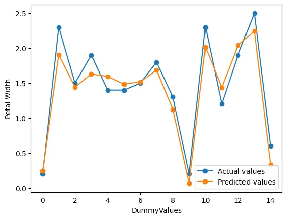

The code is quite self-explanatory. Still, I’ll explain a little about what we did here. This is multivariate linear regression. I took the ‘Sepal_length’, ‘Sepal_width’, and ‘Petal_length’ as my inputs or independent variables and tried to predict the corresponding ‘Petal_width’. As you can see from the output, the predicted values of petal width are quite close to the actual values. Lastly, I’ve plotted a figure to show visually how good the predictions are by comparing them with the actual data. The figure shows that our linear regression model performs quite well when considering how little effort it took to implement it.

Clustering

Now that we’ve talked extensively about supervised learning implementations, let’s move onto a brief introduction to unsupervised learning implementation. We’ll only cover the clustering task for unsupervised machine learning. As mentioned earlier, one form of unsupervised learning is called clustering, where the input data is clustered or grouped together based on their similarity. It is based on discovering some features or patterns that already exist within the input data.

Clustering algorithms work with unlabeled data and try to group them by defining a similarity index and then checking the similarity between all the data points. Similar data points are then put into the same group, while the dissimilar samples are put into different groups.

As we’ve mentioned, there are several clustering algorithms, including K-Means, Hirearchial clustering, etc.

Clustering dataset: Iris dataset

The Iris dataset can also be used for clustering. As we already know, the Iris dataset has three classes of Iris species; we may use the input features, such as sepal length and sepal width, to cluster them into three groups. We might need to standardize the dataset since some clustering algorithms do not perform well if the data is not somewhat normally distributed (with 0 mean and one variance).

Clustering with sklearn

Let’s implement clustering with sklearn. We will only cover the K-Means clustering algorithm in this article.

K-Means clustering

I explained how K-means algorithm works briefly in one of the previous sections. Now, I’ll explain how it works in a simple fashion using an example:

Let’s take six integer values as our input data: [1, 2, 3, 7, 8, 9]. We have to provide the number of clusters/groups as the parameter for K-Means. Let’s say we take K = 2, which will divide the input data into two groups. Now K-Means algorithm will take two centroids randomly from the input data. Let’s assume the centroids are 3 (centroid1) and 8 (centroid2). Now each input data point will be considered, and their distance from the centroids will be calculated. The absolute distances (no negative values) from centroid1 (3) are [2, 1, 0, 4, 5, 6] and the distances from centroid2 (8) are [7, 6, 5, 1, 0, 1] for each value of the input dataset. We can easily see that the dataset closest to centroid1 (3) is [1, 2, 3], and for centroid2 (8), the closest dataset is [7, 8, 9]. Now K-means has divided the data into two clusters; however, it will refine its centroids to see if there are other ways to cluster the datapoints better. For the first group [1, 2, 3], the mean or the centroid is 2, and for the second group [7, 8, 9], the mean is 8. Using these recalculated new centroids, when we try to iterate again or cluster again, these clusters do not change, i.e., the final clusters would be [1, 2, 3] and [7, 8, 9] with centroids 2 and 8.

Now let’s use sklearn to perform linear regression on the Iris dataset:

# Import necessary modules
from sklearn import datasets
from sklearn.preprocessing import MinMaxScaler
from sklearn.model_selection import train_test_split
from sklearn.cluster import KMeans
from sklearn.metrics import accuracy_score
from sklearn.metrics import classification_report
import pandas as pd
from matplotlib import pyplot as plt
%matplotlib inline

# Load the Iris dataset
iris = datasets.load_iris()
X_iris = iris["data"]  # input features
y_iris = iris["target"]  # labels

# Copy the dataset to a pandas DataFrame
df_iris = pd.DataFrame(X_iris, columns = ['Sepal_length','Sepal_width','Petal_length','Petal_width'])
df_iris['Species'] = y_iris

# Visualize the data
bx = df_iris[df_iris.Species==0].plot.scatter(x='Petal_length', y='Petal_width', color='red', label='Iris - Setosa')
df_iris[df_iris.Species==1].plot.scatter(x='Petal_length', y='Petal_width', color='green', label='Iris - Versicolor', ax=bx)
df_iris[df_iris.Species==2].plot.scatter(x='Petal_length', y='Petal_width', color='blue', label='Iris - Virginica', ax=bx)
bx.set_title("Petal width (cm) vs Petal length (cm) for 3 Iris species")

Text(0.5, 1.0, 'Petal width (cm) vs Petal length (cm) for 3 Iris species')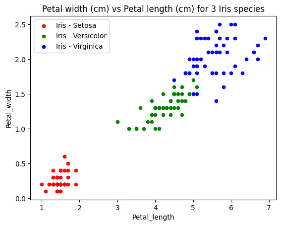

In this section of the code, we load the Iris dataset like the other times. This time we visualize the data, specifically, we take a look at the petal width vs petal length graph. As we can see, the data is in clusters for each of the species. Now let’s apply K-Means to our dataset:

# Cluster using KMeans
clstr = KMeans(n_clusters=3, init='k-means++', random_state=0)

# Fit KMeans and make predictions on the test set and print
y_pred = clstr.fit_predict(X_iris)
print(y_pred)

# Plot the clusters found by KMeans
plt.scatter(X_iris[y_pred==0,2], X_iris[y_pred==0,3], s = 15, c= 'green', label = 'Cluster_1')
plt.scatter(X_iris[y_pred==1,2], X_iris[y_pred==1,3], s = 15, c= 'red', label = 'Cluster_2')
plt.scatter(X_iris[y_pred==2,2], X_iris[y_pred==2,3], s = 15, c= 'blue', label = 'Cluster_3')
plt.legend()

[1 1 1 1 1 1 1 1 1 1 1 1 1 1 1 1 1 1 1 1 1 1 1 1 1 1 1 1 1 1 1 1 1 1 1 1 1
 1 1 1 1 1 1 1 1 1 1 1 1 1 0 0 2 0 0 0 0 0 0 0 0 0 0 0 0 0 0 0 0 0 0 0 0 0
 0 0 0 2 0 0 0 0 0 0 0 0 0 0 0 0 0 0 0 0 0 0 0 0 0 0 2 0 2 2 2 2 0 2 2 2 2
 2 2 0 0 2 2 2 2 0 2 0 2 0 2 2 0 0 2 2 2 2 2 0 2 2 2 2 0 2 2 2 0 2 2 2 0 2
 2 0]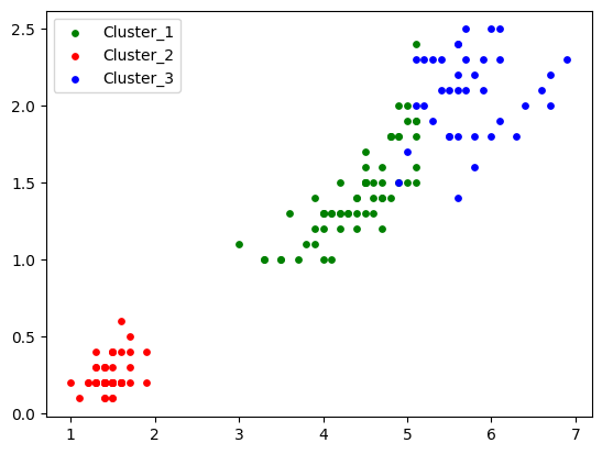

After running K-Means to our dataset, we can see the predictions in the output (remember not to confuse yourself with the numbers associated with the clusters [0, 1, 2] and the numbers representing the species or y_iris [0, 1, 2]. They are not the same. This is because k-Means randomly assigns the numbers associated with the clusters.)

We also notice from the figure that the K-Means clustering performs quite well, separating the data into three groups or clusters. Let’s plot the original dataset and clustered dataset, stacking them vertically:

# Plot dataset and show KMeans clustering vertically stacked
fig, axs = plt.subplots(2)
fig.suptitle('Performance of KMeans Clustering')

axs[0].scatter(X_iris[y_iris==0,2], X_iris[y_iris==0,3], s = 15, c= 'red', label = 'Iris - Setosa')
axs[0].scatter(X_iris[y_iris==1,2], X_iris[y_iris==1,3], s = 15, c= 'green', label = 'Iris - Versicolor')
axs[0].scatter(X_iris[y_iris==2,2], X_iris[y_iris==2,3], s = 15, c= 'blue', label = 'Iris - Virginica')
axs[0].legend()

axs[1].scatter(X_iris[y_pred==0,2], X_iris[y_pred==0,3], s = 15, c= 'green', label = 'Cluster_1')
axs[1].scatter(X_iris[y_pred==1,2], X_iris[y_pred==1,3], s = 15, c= 'red', label = 'Cluster_2')
axs[1].scatter(X_iris[y_pred==2,2], X_iris[y_pred==2,3], s = 15, c= 'blue', label = 'Cluster_3')
axs[1].legend()

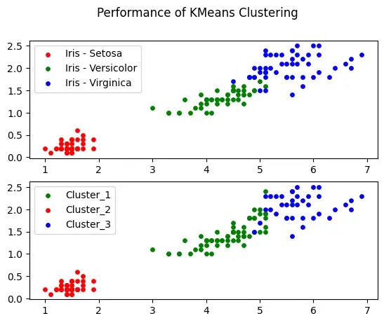
This figure tells us how closely the K-Means clustering algorithm divided the input dataset into a cluster/group of three.

Now you may wonder how we can know the value of K or the number of clusters (n_clusters) beforehand. There may be some data where you don’t know how many clusters it has; after all, K-Means is an unsupervised learning algorithm. There are multiple ways to figure out the number of clusters in a dataset. One of the most popular ways is looking at an “elbow plot.” Here’s what an elbow plot looks like [source: https://devindeep.com/kmeans-elbow-method-tutorial/]:

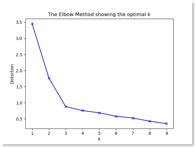
In elbow plots, we increase the value of K or the number of clusters (in the x-axis) and look at the cost function’s value (in the y-axis). There’s a point (K = 3) where the graph looks like it has a bend or angle, like at our elbow. Generally, that is the optimum value of K (in this plot, optimum K = 3). After this optimum value, the cost does not reduce significantly with increasing values of K.

Conclusion

In summary, scikit-learn is an essential tool for anybody interested in machine learning, from those just starting out to those with years of experience wishing to apply sophisticated models. It’s a robust, user-friendly library that offers several machine learning algorithms and may be put to use in many different contexts. We covered the basics of how to implement machine learning using scikit-learn or sklearn. We demonstrated examples of classification, regression, and clustering tasks. Now it’s your turn to explore the vast and exciting world of machine learning. Why hold off? Get into machine learning now using scikit-learn and see what all the fuss is about.